Présentation des architectures informatiques et des outils logiciels permettant de faciliter le traitement de données volumineuses.
Dérouler les slides ci-dessous ou cliquer ici pour afficher les slides en plein écran.
The big data phenomenon is now well-documented: the generation and collection of data from a multitude of sources (IoT sensors, daily interactions on social media, online transactions, mobile devices, etc.) drastically increases the volume of data available for analysis. There are many reasons to focus on such data in data science projects: high availability, greater granularity of observed phenomena, and large datasets needed for training increasingly data-hungry models (like LLMs), among others.
Big data is often defined as a situation where the data volume is so large that it can no longer be processed on a single machine. This relative definition may seem reductive but has the advantage of highlighting that a data source, depending on the time and environment, may require different skill sets. Moving to big data is not just a matter of scale—it often involves a fundamental shift in the computing infrastructure, with strong implications for the expertise required and the scalability of the data pipelines.
Processing such data introduces new challenges, often summarized as the “three Vs”, a widely accepted way to characterize these data sources (Sagiroglu and Sinanc 2013):
Volume: Massive volumes of data, often far beyond the capabilities of traditional systems. New storage and processing architectures are needed to handle such scales.
Velocity: These data are typically produced at high frequency, even in real time. This demands adjustments to architecture and processing methods, such as stream processing.
Variety: These data come from a wide range of sources and formats, from structured tables to unstructured data like text, images, or video. The appropriate processing techniques depend heavily on the data type. In this course, we focus on relatively structured data, as they remain central to analytical data science projects.
When considering putting a data science project based on large datasets into production, adopting good development practices is not just recommended—it is essential. Massive datasets introduce significant complexity at every stage of the data science project lifecycle, from collection and storage to processing and analysis. Systems must be designed not only to handle the current data load but also to be scalable for future growth. Good practices enable this scalability by promoting modular architectures, reusable code, and technologies suited for large-scale data processing.
To address these challenges, technology choices are crucial. In this course, we will focus on three main aspects to guide those choices: computing infrastructure, data formats suited for high volumes, and frameworks (software solutions and their ecosystems) used for data processing.
Infrastructures
Evolution of Data Infrastructures
Historically, data has been stored in databases, systems designed to store and organize information. These systems emerged in the 1950s and saw significant growth with relational databases in the 1980s. This technology proved especially effective for organizing corporate “business” data and served as the foundation of data warehouses, long considered the standard for data storage infrastructure (Chaudhuri and Dayal 1997). While technical implementations can vary, their core idea is simple: data from various heterogeneous sources is integrated into a relational database system according to business rules via ETL (extract-transform-load) processes, making it accessible for a range of uses (statistical analysis, reporting, etc.) using the standardized SQL language (Figure 1).
Figure 1: Architecture of a data warehouse. Source: airbyte.com
In the early 2000s, the growing adoption of big data practices exposed the limitations of traditional data warehouses. On one hand, data increasingly came in diverse formats (structured, semi-structured, and unstructured), often evolving as new features were added to data collection platforms. These dynamic, heterogeneous formats fit poorly with the ordered nature of data warehouses, which require schemas to be defined a priori. To address this, data lakes were developed—systems that allow for the collection and storage of large volumes of diverse data types (Figure 2).
Figure 2: Architecture of a data lake. Source: cartelis.com
Additionally, the enormous size of these data sets made it increasingly difficult to process them on a single machine. This is when Google introduced the MapReduce paradigm (Ghemawat, Gobioff, and Leung 2003; Dean and Ghemawat 2008), which laid the foundation for a new generation of distributed data processing systems. Traditional infrastructures used vertical scalability—adding more powerful or additional resources to a single machine. However, this quickly became expensive and hit hardware limits. Distributed architectures use horizontal scalability: by using many parallel, lower-powered servers and adapting algorithms to this distributed logic, massive datasets can be processed using commodity hardware. This led to the emergence of the Hadoop ecosystem, combining complementary technologies: a data lake (HDFS - Hadoop Distributed File System), a distributed processing engine (MapReduce), and tools for data integration and transformation (Figure 3). This ecosystem expanded with tools like Hive (which converts SQL queries into distributed MapReduce tasks) and Spark (which overcomes certain technical limitations of MapReduce and provides APIs in multiple languages, including Java, Scala, and Python). Hadoop’s success was profound—it enabled organizations to process petabyte-scale datasets in real-time using widely accessible programming languages.
This technological shift fueled the big data revolution, enabling new types of questions to be answered using vast datasets. Philosophically, it marked a shift from collecting only the data needed for known purposes, to storing as much data as possible and evaluating its usefulness later during analysis. This approach is typical of NoSQL environments (“Not only SQL”), where data is stored at each transactional event but in more flexible formats than traditional databases. JSON, derived from web transactions, is especially prominent. Depending on the structure of the data, different tools are used to query it: ElasticSearch or MongoDB for text data, Spark for tabular data, and so on. All these tools share a common trait: they are highly horizontally scalable, making them ideal for server farms.
Figure 3: Schematic of a Hadoop architecture. Large datasets are split into blocks, and both storage and processing are distributed across multiple compute nodes. Algorithms are adapted to this distributed setup via MapReduce: first, a “map” function is applied to each block (e.g., count word frequencies), then a “reduce” step aggregates these results (e.g., compute total frequencies across blocks). Output data is often much smaller than input data and can be brought back locally for further tasks like visualization. Source: glennklockwood.com
By the late 2010s, Hadoop architectures began to decline in popularity. In traditional Hadoop setups, storage and compute are co-located by design: data segments are processed on the servers where they are stored, avoiding network traffic. This architecture scales linearly, increasing both storage and compute capacity—even if only one is needed. In a provocative article titled “Big Data is Dead” (Tigani 2023), Jordan Tigani (one of the founding engineers of Google BigQuery) argues that this model no longer suits modern data workloads. First, he explains, “in practice, data size grows much faster than compute needs.” Most use cases don’t require querying all stored data—just recent subsets or specific columns. Second, “the big data frontier keeps receding”: thanks to more powerful and cheaper servers, fewer workloads require distributed systems (Figure 4). Additionally, new storage formats (see Section 2) make data handling more efficient. As a result, properly decoupling storage from compute often leads to simpler, more efficient infrastructures.
Figure 4: “The big data frontier keeps receding”: the share of data workloads that cannot be handled by a single machine has steadily declined. Source: motherduck.com
The Role of Cloud Technologies
Building on Tigani’s analysis, we observe a growing shift toward more flexible, loosely coupled architectures. The rise of cloud technologies has been pivotal in this transition, for several reasons. Technically, network latency is no longer the bottleneck it was during Hadoop’s heyday, making the co-location of compute and storage less necessary. In terms of usage, it’s not just that data volumes are growing—it’s also the diversity of data and processing needs that is expanding. Modern infrastructures must support various data formats (from structured tables to unstructured media) and a wide range of compute requirements—from parallel data processing to deep learning on GPUs (Li et al. 2020).
Two cloud-native technologies have become central to this modern flexibility: containerization and object storage. Containerization ensures reproducibility and portability—crucial for production environments—and will be discussed in the Portability and Deployment chapters. In this section, we focus on object storage, the default standard in modern data infrastructures.
Since containers are stateless by nature, a persistent storage layer is needed to store input and output data across computations (Figure 5). In container-based infrastructures, object storage has become dominant—popularized by Amazon’s S3 (Simple Storage Service) (Mesnier, Ganger, and Riedel 2003; Samundiswary and Dongre 2017). To understand its popularity, it’s helpful to contrast object storage with other storage types.
There are three main storage models: file systems, block storage, and object storage (Figure 5). File systems organize data in a hierarchical structure—like a traditional desktop environment—but they don’t scale well and require manual access management. Block storage, like that on hard drives, offers fast low-latency access—ideal for databases—but also struggles with scalability and cost. Object storage, on the other hand, breaks data into “objects” stored in a flat namespace and assigned unique IDs and metadata. It removes the need for hierarchical structures, lowering storage costs.
Figure 5: Comparison of storage types. Source: bytebytego.com
Object storage’s characteristics make it ideal for containerized data science infrastructures. It’s highly scalable, supports large files, and works well with distributed systems. It also enhances user autonomy by exposing data via APIs like Amazon’s S3, allowing direct interaction from code (R, Python, etc.) and fine-grained access control via tokens. Most importantly, object storage supports decoupled architectures, where compute and storage are independent and remotely accessible. This improves flexibility and efficiency.
Figure 6: In container-based infrastructure (which is stateless by nature), object storage provides the persistence layer. MinIO is an open-source object storage solution that integrates natively with Kubernetes and supports the S3 API—now the industry standard—ensuring compatibility across environments. Source: lemondeinformatique.fr
Data Formats
Another major dimension to consider for processing massive datasets is how data is stored. Choosing a data format involves balancing several factors, such as the purpose (processing, analysis, dissemination), the target audience (general public, project members, etc.), volume, and interoperability. Traditional formats like CSV, JSON, and XML are widely used due to their convenience: they are plain text formats, making them easily viewable in any text editor — they are considered human-readable. Additionally, they are naturally interoperable: plain text can be read by almost any programming language, and most libraries provide built-in support for reading these formats. However, these formats quickly show their limitations when dealing with massive datasets. The lack of compression results in high disk usage, and their row-based representation (Figure 7) on disk and in memory makes them inefficient — you often need to load the entire file into memory to perform operations on specific rows or columns.
One of the major innovations in the data ecosystem over the past decade is the emergence of data formats that address the limitations of traditional formats. The most popular and now standard format for data storage is Apache Parquet. It offers several features that make it especially well-suited for data science applications. First, it is a compressed format, making it ideal for storing large datasets. Depending on data structure, it’s not uncommon for a dataset in Parquet format to take up 10 times less space than its CSV equivalent. Second, Parquet is interoperable: files in this format can be queried not only with common languages like Python, R, or SQL, but also with big data processing tools like Spark.
However, the key reason for Parquet’s widespread adoption in data science is its read performance. Intuitively, one might expect that a compressed format would be slower to read than a text format like CSV—after all, decompressing takes time. But Parquet uses highly optimized compression that actually outperforms reading from a plain CSV file. A crucial feature of Parquet that contributes to this performance is that it is column-oriented, meaning data is stored by columns rather than by rows as in traditional text formats (Figure 7). This makes it highly efficient for analytical workloads (also known as OLAP — Online Analytical Processing), which often involve selecting specific columns, computing derived variables, and aggregating data by groups. Row-based formats like CSV require reading the entire dataset into memory to execute such queries. In contrast, columnar formats allow reading only the relevant columns, significantly reducing read and compute times for analytics tasks (Abdelaziz et al. 2023). In practice, popular columnar formats like Parquet use a hybrid approach: they are mainly column-oriented, but also include row-grouping techniques to further optimize filtering operations.
Figure 7: Row-based vs column-based data storage representation.
Another important feature of the Parquet format is its native support for partitioned files, which means a dataset can be split across multiple files based on one or more partition keys. In most statistical processing, the entire dataset isn’t required at once — you typically filter by geographic area, time window, etc. If all data is stored in a single file, you’d still need to load all rows — at least the relevant columns — into memory to perform such filtering. With Parquet, datasets can be partitioned by frequently used filters — similar to indexes in a SQL database — enabling much faster and more efficient queries (Figure 8). This feature makes Parquet especially well-suited for analytical tasks common in data science(Dondon and Lamarche 2023).
Figure 8: Filesystem representation of a Parquet file partitioned by two keys: year and month. In this example, querying only a few months is highly efficient because only the relevant partitions are loaded into memory.
Processing Frameworks
The Parquet format makes tabular data storage significantly more efficient. But to fully benefit from this structure, one must also consider the next step: in-memory data processing.
Two major tools have emerged in recent years to address this need. The first is Apache Arrow, an in-memory tabular data format interoperable across many languages (Python, R, Java, etc.). The second is DuckDB, a portable and interoperable database engine capable of querying highly diverse data sources (Figure 10). While technically quite different in their implementations, both tools offer similar advantages and performance gains. First, both are column-oriented and thus work synergistically with the Parquet format by preserving the benefits of columnar storage in memory (Figure 9).
Figure 9: In-memory representation of data in Arrow format. With this format, in-memory storage is also columnar. This preserves the storage advantages of Parquet in memory and leverages modern CPU improvements in vectorized operations. In this example, filtering the session_id column is significantly more efficient than in traditional row-based in-memory formats.
Moreover, both Arrow and DuckDB drastically improve query performance through lazy evaluation. While most programming languages execute data operations sequentially — e.g., select columns, filter rows, compute new variables, then perform aggregations — Arrow and DuckDB use a precomputed execution plan that globally optimizes the processing chain. This approach not only makes computations faster, but also more efficient, as only the necessary data is retrieved and processed. These innovations make it feasible to work with datasets that exceed the available RAM on a machine.
Figure 10: A major strength of DuckDB is its ability to query a wide range of data sources in a standardized way. Since DuckDB is an in-memory database engine, it is naturally suited for querying relational databases (e.g., PostgreSQL, MySQL). But it can also query data files like CSV and Parquet, whether local or cloud-hosted.
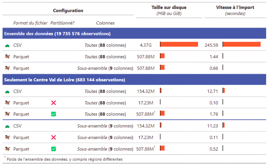
The best way to appreciate the benefits of the Parquet format is to test it and compare it against the same data stored as CSV, as shown in Figure 11. The applications below illustrate the previously mentioned concepts (lazy evaluation, partitioning, etc.) and demonstrate the usability of the Arrow and DuckDB ecosystems through simple examples. The capstone application covers Parquet in less detail.
Figure 11: Example performance comparison of the Parquet format in various use cases using detailed population census data released by Insee in 2023
Applications
Throughout this application, we will explore how to use the Parquet format as efficiently as possible. To compare different formats and usage methods, we will compare execution time and memory usage for a standard query. Let’s start with a small dataset example to compare the CSV and Parquet formats.
To do this, we need to retrieve some data in Parquet format. We suggest using detailed and anonymized population census data from France: about 20 million rows and 80 columns. The code to retrieve the data is given below
Code
import pyarrow.parquet as pqimport pyarrow as paimport os# Définir le fichier de destinationfilename_table_individu ="data/RPindividus.parquet"# Copier le fichier depuis le stockage distant (remplacer par une méthode adaptée si nécessaire)1os.system("mc cp s3/projet-formation/bonnes-pratiques/data/RPindividus.parquet data/RPindividus.parquet")# Charger le fichier Parquettable = pq.read_table(filename_table_individu)df = table.to_pandas()# Filtrer les données pour REGION == "24"df_filtered = df.loc[df["REGION"] =="24"]# Sauvegarder en CSVdf_filtered.to_csv("data/RPindividus_24.csv", index=False)# Sauvegarder en Parquetpq.write_table(pa.Table.from_pandas(df_filtered), "data/RPindividus_24.parquet")
1
This line of code uses the Minio Client utility available on the SSPCloud. If you are not on this infrastructure, you can refer to the dedicated warning
There are several ways to do this. For example, you can use pure Python with requests. If you have curl installed, you can also use it. Via Python, this would be the command os.system("curl -o data/RPindividus.parquet https://projet-formation/bonnes-pratiques/data/RPindividus.parquet").
These exercises will use Python decorators, i.e., functions that override the behavior of another function. In this case, we will create a function that runs a chain of operations and override it with another one that monitors memory usage and execution time.
Part 1: From CSV to Parquet
Create a notebook benchmark_parquet.ipynb to perform various performance comparisons for the application.
Let’s create our decorator, responsible for benchmarking the Python code:
Dérouler pour retrouver le code du décorateur permettant de mesurer la performance
The following query calculates the data needed to build a population pyramid for a given department, using the census CSV file. Test it in your notebook:
Dérouler pour récupérer le code de lecture du CSV
import pandas as pd# Charger le fichier CSVdf = pd.read_csv("data/RPindividus_24.csv")res = ( df.loc[df["DEPT"] ==36] .groupby(["AGED", "DEPT"])["IPONDI"] .sum().reset_index() .rename(columns={"IPONDI": "n_indiv"}))
Repeat this code to encapsulate these operations in a process_csv_appli1 function:
Dérouler pour récupérer le code pour mesurer les performances de la lecture en CSV
# Apply the decorator to functions@measure_performancedef process_csv_appli1(*args, **kwargs): df = pd.read_csv("data/RPindividus_24.csv")return ( df.loc[df["DEPT"] ==36] .groupby(["AGED", "DEPT"])["IPONDI"] .sum().reset_index() .rename(columns={"IPONDI": "n_indiv"}) )
Run process_csv_appli1() and process_csv_appli1(return_output=True)
Following the same model, build a process_parquet_appli1 function based this time on the file data/RPindividus_24.parquet loaded with Pandas’ read_parquet function.
Compare the performance (execution time and memory allocation) of these two methods using the function.
❓️ What seems to be the limitation of the read_parquet function?
We already save a significant amount of time on reading, but we don’t fully benefit from the optimizations enabled by Parquet because we immediately transform the data into a PandasDataFrame after reading it. This means we are not using one of Parquet’s key features that explains its excellent performance: predicate pushdown, which optimizes processing by applying filters on columns as early as possible to retain only those actually used in the operation.
Part 2: Leveraging lazy evaluation and Arrow or DuckDB optimizations
The previous section showed a significant time gain when switching from CSV to Parquet. However, memory usage remained very high, even though only a small portion of the file was actually used.
In this section, we’ll explore how to use lazy evaluation and execution plan optimizations performed by Arrow to fully harness the power of the Parquet format.
Open the file data/RPindividus_24.parquet with pyarrow.dataset. Check the class of the resulting object.
Try the code below to read a data sample:
( dataset.scanner() .head(5) .to_pandas())
Do you understand the difference compared to before? Look at the documentation for the to_table method: do you grasp its purpose?
Build a function summarize_parquet_arrow (or summarize_parquet_duckdb) which now imports the data using the pyarrow.dataset function (or with DuckDB) and performs the desired aggregation.
Compare the performance (execution time and memory allocation) of the three methods (Parquet read and processed with Pandas, Arrow, and DuckDB) using our function.
Code complet de l’application
import duckdbimport pyarrow.dataset as ds@measure_performancedef summarize_parquet_duckdb(*args, **kwargs): con = duckdb.connect(":memory:") query =""" FROM read_parquet('data/RPindividus_24.parquet') SELECT AGED, DEPT, SUM(IPONDI) AS n_indiv GROUP BY AGED, DEPT """return (con.sql(query).to_df())@measure_performancedef summarize_parquet_arrow(*args, **kwargs): dataset = ds.dataset("data/RPindividus_24.parquet", format="parquet") table = dataset.to_table() grouped_table = ( table .group_by(["AGED", "DEPT"]) .aggregate([("IPONDI", "sum")]) .rename_columns(["AGED", "DEPT", "n_indiv"]) .to_pandas() )return ( grouped_table )process_parquet()summarize_parquet_duckdb()summarize_parquet_arrow()
With lazy evaluation, the process unfolds in multiple stages:
Arrow or DuckDB receives instructions, optimizes them, and executes the queries
Only the output data from this chain is sent back to Python
Application 3
Part 3a: What if we filter rows?
Add a row filtering step in our queries:
With DuckDB, modify the query with WHERE DEPT IN ('18', '28', '36')
With Arrow, modify the to_table step as follows: dataset.to_table(filter=pc.field("DEPT").isin(['18', '28', '36']))
Correction de cet exercice
import pyarrow.dataset as dsimport pyarrow.compute as pcimport duckdb@measure_performancedef summarize_filter_parquet_arrow(*args, **kwargs): dataset = ds.dataset("data/RPindividus.parquet", format="parquet") table = dataset.to_table(filter=pc.field("DEPT").isin(['18', '28', '36'])) grouped_table = ( table .group_by(["AGED", "DEPT"]) .aggregate([("IPONDI", "sum")]) .rename_columns(["AGED", "DEPT", "n_indiv"]) .to_pandas() )return ( grouped_table )@measure_performancedef summarize_filter_parquet_duckdb(*args, **kwargs): con = duckdb.connect(":memory:") query =""" FROM read_parquet('data/RPindividus_24.parquet') SELECT AGED, DEPT, SUM(IPONDI) AS n_indiv WHERE DEPT IN ('11','31','34') GROUP BY AGED, DEPT """return (con.sql(query).to_df())summarize_filter_parquet_arrow()summarize_filter_parquet_duckdb()
❓️ Why don’t we save time with row filters (or even lose time), unlike with column filters?
Data is not organized in row blocks the way it is in column blocks. Fortunately, there’s a way around this: partitioning!
Part 3: Partitioned Parquet
Lazy evaluation and Arrow optimizations already bring considerable performance gains. But we can do even better! When we know that data will regularly be filtered based on a specific variable, it is a good idea to partition the Parquet file by that variable.
Browse the documentation for pyarrow.parquet.write_to_dataset to understand how to specify a partitioning key when writing a Parquet file. Several methods are possible.
Import the full census individual table from "data/RPindividus.parquet" using pyarrow.dataset.dataset and export it as a partitioned table to "data/RPindividus_partitionne.parquet", partitioned by region (REGION) and department (DEPT).
Examine the file tree structure of the exported table to see how the partitioning was applied.
Modify the import, filtering, and aggregation functions using Arrow or DuckDB to now use the partitioned Parquet file. Compare this to using the non-partitioned file.
Answer to question 2 (writing the partitioned Parquet)
A workshop on the Parquet format and DuckDB ecosystem for EHESS, with R and Python examples using the same data source as this application.
The getting started guide for census data in Parquet format with examples using DuckDB in WASM (directly in the browser, without R or Python installation).
References
Abdelaziz, Abdullah I, Kent A Hanson, Charles E Gaber, and Todd A Lee. 2023. “Optimizing Large Real-World Data Analysis with Parquet Files in r: A Step-by-Step Tutorial.”Pharmacoepidemiology and Drug Safety.
Chaudhuri, Surajit, and Umeshwar Dayal. 1997. “An Overview of Data Warehousing and OLAP Technology.”ACM Sigmod Record 26 (1): 65–74.
Dean, Jeffrey, and Sanjay Ghemawat. 2008. “MapReduce: Simplified Data Processing on Large Clusters.”Communications of the ACM 51 (1): 107–13.
Dondon, Alexis, and Pierre Lamarche. 2023. “Quels Formats Pour Quelles Données?”Courrier Des Statistiques, 86–103.
Ghemawat, Sanjay, Howard Gobioff, and Shun-Tak Leung. 2003. “The Google File System.” In Proceedings of the Nineteenth ACM Symposium on Operating Systems Principles, 29–43.
Li, Yun, Manzhu Yu, Mengchao Xu, Jingchao Yang, Dexuan Sha, Qian Liu, and Chaowei Yang. 2020. “Big Data and Cloud Computing.”Manual of Digital Earth, 325–55.
Mesnier, Mike, Gregory R Ganger, and Erik Riedel. 2003. “Object-Based Storage.”IEEE Communications Magazine 41 (8): 84–90.
Sagiroglu, Seref, and Duygu Sinanc. 2013. “Big Data: A Review.” In 2013 International Conference on Collaboration Technologies and Systems (CTS), 42–47. IEEE.
Samundiswary, S, and Nilma M Dongre. 2017. “Object Storage Architecture in Cloud for Unstructured Data.” In 2017 International Conference on Inventive Systems and Control (ICISC), 1–6. IEEE.